“Buy low, sell high”. Everyone’s heard of that one. In fact, we’ve probably all heard it so much we no longer have to think about the math behind it, we just *know* that means you’ve made money. There are some things you don’t even have to think about any more, you just feel them. “Your average income tax rate is not the same as your marginal income tax rate”. That one requires a little more thought, but yes, it makes sense; only the amount of taxable income that falls in the highest marginal bracket is taxed at that rate; the rest is taxed according to lower tax brackets, and at the end of it all your average tax rate is a blend of what you’re paying for all the different tax brackets. Phew! That was a little more heavy lifting, but still, we’ve seen it enough where we understand it.
So why, then, are portfolio returns seemingly so tricky? Why do most people believe that if they lose 5% and then make 5% back, they would be at break-even? After all, the average of -5 and 5 is still 0, right? Well, not always. Let’s look at the math.
First, the 5% loss: $100 x (1 – .05) = $95. So far, so good.
Now, the 5% gain: $95 x (1 + .05) = $99.75.
And there you have it. Were you to lose 5% and then gain 5% back, you’d be out 0.25%. Even when you start with the 5% gain and then suffer a 5% loss, you still end up losing 0.25%. This cruel little twist of math is why losses are worth minimizing: losses do more harm to investments than gains of the same order of magnitude help. Sure, a 0.25% loss isn’t all that big of a deal; it’s practically no loss at all. This brings us to our second bit of cruel math: the larger the loss, the harder it is to get back to break-even.
Let’s look at the same loss and gain situation, but with a larger return factor of 20%:
$100 x (1 – .2) = $80; $80 x (1 + .2) = $96.
Down 20% and up 20% leaves you 4% short, which still isn’t that big of a loss, but by the time you get to a 40% loss and 40% gain, you’re out 16%. As you continue to lose, it gets harder and harder to make it back, and by the time you’re down 50%, you need a 100% gain to get back to break-even. The bigger the ups and downs, the more volatile the situation. If you remember last month’s piece on volatility called “How to Play with Fire”, you know that volatility is something that requires managing, and now you can see the math behind why that is.
The takeaways here are that even though the simple average of -5% and 5% is 0%, you do not get back to break-even when your investments experience those returns. Likewise, even though both -5% and 5%, and -20% and 20% have a simple average of 0%, the impact on your investments is not the same when experiencing those particular loss and gain combinations; down and up 20% leaves you worse off than down and up 5%.
Here’s an important point on terminology. We use terms like “average return”, “annual return”, or “average annual returns” quite frequently in our monthly pieces. What we have been discussing here is the “average of returns”. In other words, add them all up and divide by how many there are. That’s a simple average. We believe this is how many people estimate their investment returns. However, that is not how the math of calculating average returns works. For example, if one portfolio makes 14% one year and 1% the next, the average of those returns is 7.5%. Another portfolio can earn 7.5% one year, 7.5% the next, and have the same average of returns, so shouldn’t their balances be equal after those two years? Actually, no. If both portfolios started with $1,000, the first would have $1,151 after two years, but the second would have $1,156. The average of their returns might be the same, but their average annual returns are different. Why couldn’t math have been so interesting when we were in 8th grade?!
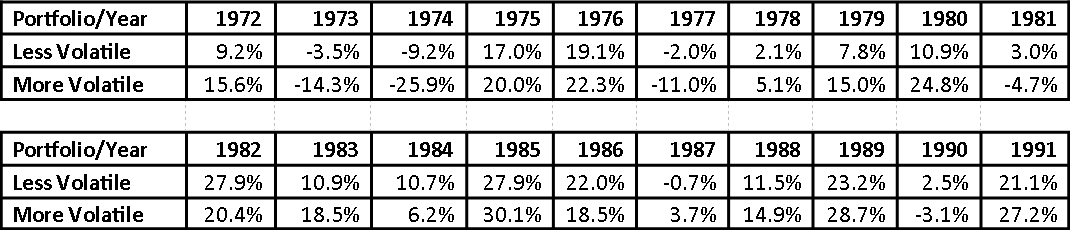
Now that we’ve done the prerequisite work on why losses matter as much as they do, let’s look at how losses work inside portfolios to compound the harm for investors. To make this analysis mirror the real world as much as possible, we’re going to look at what two 40% bond, 60% stock portfolios returned over a 20 year period from 1972 – 1991. Each tracks the ups and downs of the stock and bond markets over that period, and both have the exact same average of returns of 10.6%. However, one portfolio is 50% more volatile than the other, which can happen when portfolios have the same general exposure to stocks and bonds but contain different specific securities. Therefore, though the portfolio with the more volatile investments experiences larger gains, it also experiences larger losses. For anyone who wants a detailed look at the annual returns of the two portfolios, they are as follows:
In this analysis, we’re going to show the effects of choosing a less volatile portfolio versus a more volatile one on a retired investor with $36,000 of fixed income from social security, annual expenses starting at $72,000, and a starting investment balance of $850,000. We’re going to inflate the income and expenses by the annual social security increases and inflation experienced between 1972 and 1991. Considering where our economy and money supply is today, using inflation metrics from the 1970’s seems appropriate. With both portfolios’ average of returns over 10% for the time period, the fact that this investor is withdrawing around 4% to meet his or her expense needs seems reasonable.
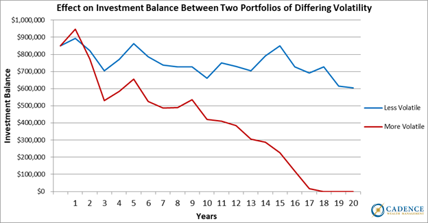
This right here is why avoiding large losses matters. Both portfolios have the same 10%+ average of returns over the 20 years, but one is more volatile and loses more during most market downturns. Even though the average of returns for both portfolios was over 10% for 20 years, the 4% distributions needed to close the expense gap were not sustainable for the portfolio with the bigger losses, even though it also had bigger gains. Even for investors who are not retired, any withdrawal, and that includes panicking and selling when investment values plummet, can lock losses in and permanently damage investment growth. Two portfolios with the same average returns can experience very different outcomes, which is why understanding some of the math behind investment losses is important. Increased volatility can lead to larger losses when investments turn negative, and even a portfolio with a higher average return can still lead to a bad outcome if the large losses come at the wrong time, or are coupled with portfolio distributions.
While not as surprising as finding out 1 + 1 doesn’t equal 2, finding out losing 5% and then making 5% back doesn’t get a portfolio back to break-even still catches most investors by surprise. Learning that two portfolios with the same average returns can lead to different outcomes is also similarly eye-opening. What losses can do to portfolios should always be taken into account when evaluating what to own at any given time, because some holes can get too deep to dig out of. Minimizing losses should be as intuitive as “buy low, sell high”, but not enough investors know the math involved. In the spirit of the back to school season we have a pop quiz to end this article:
Question: When is the best time to minimize your investment losses?
Answer: Before they happen.
Editors Note: This article was originally published in the October 2020 edition of our “Cadence Clips” newsletter.
Important Disclosures
This blog is provided for informational purposes and is not to be considered investment advice or a solicitation to buy or sell securities. Cadence Wealth Management, LLC, a registered investment advisor, may only provide advice after entering into an advisory agreement and obtaining all relevant information from a client. The investment strategies mentioned here may not be suitable for everyone. Each investor needs to review an investment strategy for his or her own particular situation before making any investment decision.
Past performance is not indicative of future results. It is not possible to invest directly in an index. Index performance does not reflect charges and expenses and is not based on actual advisory client assets. Index performance does include the reinvestment of dividends and other distributions
The views expressed in the referenced materials are subject to change based on market and other conditions. These documents may contain certain statements that may be deemed forward‐looking statements. Please note that any such statements are not guarantees of any future performance and actual results or developments may differ materially from those projected. Any projections, market outlooks, or estimates are based upon certain assumptions and should not be construed as indicative of actual events that will occur. Data contained herein from third party providers is obtained from what are considered reliable sources. However, its accuracy, completeness or reliability cannot be guaranteed.
Examples provided are for illustrative purposes only and not intended to be reflective of results you can expect to achieve.